On June 25, 2012, TIA’s CEO and founder, Sheila Weinberg, and others gave testimony before GASB which impacted its approval of new accounting standards for pensions by employers.
GASB Statement No. 67 (effective in the 2014 fiscal year) will require state pension plans to report their total NPL. This NPL is the difference between Total Pension Liability (TPL) and Fiduciary Net Position (FNP) (i.e. market value of assets).
Once a pension plan is projected to run out of assets, the pension liabilities must be valued using a “blended” discount rate. This lower rate will result in significant increases in these liabilities.
GASB Statement No. 68 (effective in the 2015 fiscal year) will require states to report the full amount of their unfunded pension liabilities on the face of their balance sheet. This will represent a major change in the reporting requirements because the vast majority of these liabilities were previously excluded from states’ financial statements. Like in TIA's previous studies, each state's financial condition was calculated as if this standard had been implemented.
The amendments are based upon the principle that: “Pensions are a form of compensation, like salaries, which governments provide in return for work” (Governmental Accounting Standards Board 2011, 54). GASB concluded from this observation that pension obligations should be recorded when earned, not when paid.
Previously, many states determined their pension plan contributions based upon the annual required contributions (ARC) calculated according to GASB’s pension standard. Whether or not the states paid these annual contributions was the largest factor used in judging if states were adequately funding their pension plans.
Under the amended statements, no ARC is required to be disclosed. The pension expense will not be an annual contribution or funding amount, rather a change in the NPL recognized from one year to the next, except for the change to actuarial assumptions (Governmental Accounting Standards Board 2011, vii). Determining whether a state is balancing its budget will be difficult with the inclusion of the pension expense on its income statement.
Additional requirements of the new standards include the following:
- The use of The American Academy of Actuarial Standards of Practice, which will likely mandate use of more realistic discount rates to calculate retirement plans’ accrued benefits and required contributions
- A standardized method to calculate accrued benefits
- A lower discount rate, based on a portfolio rate of municipal securities, should be used for the unfunded portion of the NPL
- A more realistic approach to the amortization of prior service costs that relates these costs to the expected remaining tenure of the employees concerned
- Incorporation and recognition of accrued benefit changes and likely cost of living benefit increases at the time they are created
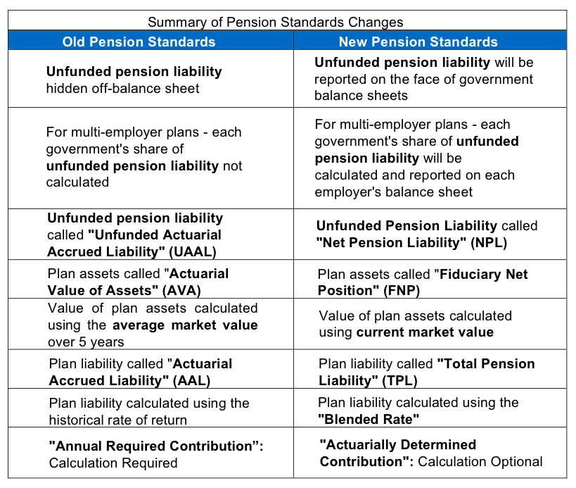
Net Pension Liability Replaces Unfunded Actuarial Accrued Liability
In similar studies, like those done by the Pew Charitable Trust and State Budget Solutions (SBS), each state's unfunded retirement liabilities were determined by allocating to the state the total unfunded liabilities of multi-employer, cost-sharing plans that the state contributed to or managed. In some cases the state contributed very little into those plans. GASB’s amendments follow TIA’s lead in requiring states to calculate and record only their share of liabilities related to these plans, based upon the contributions the state makes into the plans on their balance sheets.
The calculation of the pension shortfall is very complicated because it relies on the estimations and predictions of the future. States pay professionals, called actuaries, to make these estimations and predictions, called actuarial assumptions.
Actuarial assumptions relate to unknown, but somewhat predictable events such as employee retirement ages, increases in the benefit structures, life expectancy, costs for future medical care, and a host of other cost drivers. Actuaries also estimate the future earning power of retirement fund assets and calculate the amount of investments needed today to have money available to pay promised benefits in the future.
The asset valuation method is an important actuarial assumption that should require serious consideration. Administrators of retirement plans have used what is called “smoothing” to calculate the value of their plan assets. Smoothing computes the value of retirement plan assets at their average market value over a period of time (usually five years) attempting to adjust for severe market gains and losses. This approach leads to less volatile reported investment earnings, but it doesn’t give the most transparent view of the financial situation. Amidst significant market declines, smoothing can result in assets being valued in excess of current market values, which may induce governments to under-fund plans over the longer term. However, going forward, Statement No. 67 will eliminate smoothing for plans when reporting their asset values.
Instead of a smoothed amount, the market value of assets at year end is used to determine the Fiduciary Net Position. As noted above, we welcome this change, as truthful accounting reflects a world where volatility is a fact of life. Artificially smoothed “actuarial asset values” can mask the risks of providing defined benefit plans. A great deal of risk is involved in offering employees’ retirement benefits under these plans, and one of the greatest sources of this risk is the fluctuation in the market value of plan assets. This risk should be highlighted, rather than hidden from the public. We are pleased to see governments moving away from smoothing. TIA's research found that the change in valuing plan assets using market value versus smoothing resulted in state plans' asset values increasing and unfunded pension liabilities decreasing. The smoothed asset values were depressed because the valuation period included years of the Great Recession. Comparisons over time will have to be careful not to mix apples and oranges (i.e. funding ratios using “smoothed” vs. current “fair” values).
Actuaries matter just as much for liability reporting as they do for asset valuation. They use “present value” calculations to estimate a plan’s future benefits, as well as the contributions needed to pay those benefits. Accounting standards use a framework where the present value of the pension and OPEB liabilities is the amount that would have to be invested today —at an assumed rate of return—to ensure money will be available to pay future benefits. The assumed rate of return is the actuarial assumption of what plan assets are expected to earn before being used to pay benefits. To calculate the present value, the estimated future payments to retirees must be discounted. Discounting is the calculation of the present value of a payment or series of payments that is to be received in the future. When discounting the future pension benefits, a higher rate of return (discount rate) leads to the estimation of a lower present value of the liability. Therefore, smaller contributions from the employer would be required to adequately fund it. Conversely, a lower discount rate results in a higher estimate of the present value of the liability, thus requiring the state to contribute more into the plan.
For any government interested in understating future obligations, this understandably could lead to an incentive to assume higher rates of return on investments (typically around 7.5%) – and therefore lower liabilities. In turn, however, some notable analysts have also concluded that practices like these can prompt higher risk-seeking behavior in investment policies. These analysts make a theoretically defensible argument that retirement benefit obligations should be valued with a much lower “risk-free” rate (the rate of return on municipal bonds, which is around 5.0%), particularly in states where benefits are protected by constitutions or statutes. Using these “risk- free” rates would lead to much higher liabilities – even higher than those that TIA adds to reported state balance sheets.
The rate of return used to calculate the assets that need to be set aside to fund promised benefits is the most important assumption used in valuing and funding a pension plan. Small differences in interest rates generate significant differences in contributions required. A 2007 United States Government Accountability Office (GAO) study highlighted significant differences that various rates of return have on the pension plan contributions. The GAO’s “higher return” scenario (6% rate of return) required contributions of 5% of salaries per year. The “base case” (5% rate of return) required contributions of 9.3% of salaries per year. The “lower-return” scenario (4% rate of return) required contributions of 13.9% of salaries per year. The “risk-free” scenario (3% rate of return) required contributions of 18.6% of salaries per year (Governmental Accounting Standards Board 2011, 28).
Many pension plan administrators have historically taken the position that pension assets are invested over a long period of time and the rate of return should be based upon the long-term return assets have historically earned. Others disagree, and debate persists whether these rates should be based on historical or projected returns – including debate over whether projected returns are really historical returns in disguise.
Going forward, however, the rules regarding appropriate discount rates are now changing with the implementation of GASB Statement No. 67. Plans that project themselves to remain solvent will use their expected future of investment return rate to discount pension obligations, similar to before. However, plans that project themselves to run out of assets will have to use a “blended” rate. This rate will be an average of a) the expected investment return in the period in which assets supporting benefits remain positive, and b) a rate based on “high-quality” municipal bond yields for the periods when benefits are promised, but there are no assets projected to stand behind the plan. At current interest rates, assuming projected returns remain in line with recent practice, a blended rate will lead to lower rates, and therefore higher liabilities for plans that project themselves to run out of assets.
Governments will have to determine if and when their retirement plans will run out of assets to pay future benefits. Most plans’ actuaries are assuming plans will not run out of assets, thus the lower blended rates were not used. Consequently, very few states saw a significant increase in their pension liabilities due to the new standard. Arizona used a blended rate only for its elected officials’ retirement plan. Colorado used a blended rate only for the judges’ portion (which is relatively small) of its major plan. Illinois used a blended rate for several of its plans, but also projected that these plans wouldn’t run out of assets for fifty years. Therefore, the discount rate did not change by much, and neither did the liabilities. However, New Jersey assumed they would run out of assets soon, and used significantly lower blended discount rates for all of its pension plans. The impact was dramatic. TIA’s calculation of its share of unfunded pension liabilities has spiked dramatically under the new standards, climbing from just under $40 billion in 2013 to almost $85 billion in 2014.
As might be expected, it isn’t always easy for a plan to project itself to run out of assets. Because declaring a fund will run out of assets means a lower rate of investment and a significantly higher liability, obvious incentives exist to understate the probability and timing of shortfalls under the new standard(s). This likely helps explain why so few plans have chosen to project any future shortfall, compared to what we were expecting under Statement No. 67.